

1 引言
2 资料来源与方法介绍
2.1 资料来源
表1 涡动相关系统各观测仪器和架设高度或埋设深度Table 1 Height or depth of the instruments related to eddy covariance system |
| 观测项目 | 观测仪器, 型号 | 高度或埋深/m |
|---|---|---|
| 三维风速 | CSAT3, Campbell | 2.7 |
| H2O/CO2浓度 | EC150, Campbell | 2.7 |
| 辐射计 | CNR1, Kipp & Zonen | 1.5 |
| 土壤温度 | 109SS, Campbell | 0.05, 0.10, 0.20, 0.40 |
| 土壤体积含水量 | CS650, Campbell | 0.05, 0.10, 0.20, 0.40 |
| 土壤热通量 | HFP01, Hukseflux | 0.025, 0.075 |
| 空气温湿度 | HMP155A, Vaisala | 2.7 |
表2 微气象观测系统各观测仪器及架设高度或埋设深度Table 2 Height or depth of the instruments related to micrometeorological measurement system |
| 观测项目 | 观测仪器, 型号 | 高度或埋深/m |
|---|---|---|
| 风向风速 | WindSonic, Gill | 1, 2, 5, 10 |
| 空气温湿度 | HMP45C, Campbell | 1, 2, 5, 10 |
| 辐射四分量 | CNR4, Kipp & Zonen | 1.5 |
| 土壤温度 | 109SS, Campbell | 0.05, 0.10, 0.20, 0.40, 0.80, 1.60 |
| 土壤体积含水量 | CS616, Campbell | 0.05, 0.10, 0.20, 0.40, 0.80, 1.60 |
| 土壤热通量 | HFP01, Hukseflux | 0.025, 0.075, 0.15, 0.30 |
| 降水量 | T200B-3, Geonor | 0.75 |
表3 感热通量、 潜热通量和净生态系统交换量缺失率Table 3 Missing rate of sensible heat flux, latent heat flux and net ecosystem exchange |
| 项目 | 1月 | 2月 | 3月 | 4月 | 5月 | 6月 | 7月 | 8月 | 9月 | 10月 | 11月 | 12月 | 全年 |
|---|---|---|---|---|---|---|---|---|---|---|---|---|---|
| gap_H | 14.5% | 16.6% | 10.3% | 10.2% | 13.9% | 9.0% | 6.9% | 8.3% | 9.8% | 9.7% | 9.9% | 12.5% | 10.7% |
| gap_LE | 18.0% | 25.2% | 15.9% | 21.4% | 28.0% | 19.4% | 18.2% | 19.1% | 28.3% | 20.5% | 14.4% | 16.2% | 20.3% |
| gap_NEE | 46.3% | 52.0% | 46.5% | 31.7% | 29.0% | 22.5% | 22.5% | 21.8% | 31.6% | 22.7% | 20.1% | 44.4% | 32.6% |
2.2 方法介绍
3 结果分析
3.1 三种机器学习算法的整体性能评估
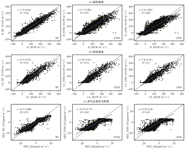
图1 S1方案下不同机器学习算法模拟的感热通量、 潜热通量和净生态系统交换量与其对应的实际观测值(M)的线性回归分析Fig.1 Linear regression analysis of observed sensible heat flux, latent heat flux and net ecosystem exchange against different machine learning algorithms simulated sensible heat flux, latent heat flux and net ecosystem exchange using gap-filling strategy S1 |
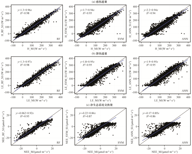
图2 S2方案下不同机器学习算法模拟的感热通量、 潜热通量和净生态系统交换量与其对应的实际观测值(M)的线性回归分析Fig.2 Linear regression analysis of observed sensible heat flux, latent heat flux and net ecosystem exchange against different machine learning algorithms simulated sensible heat flux, latent heat flux and net ecosystem exchange using gap-filling strategy S2 |
3.2 插补效果的时间变化特征
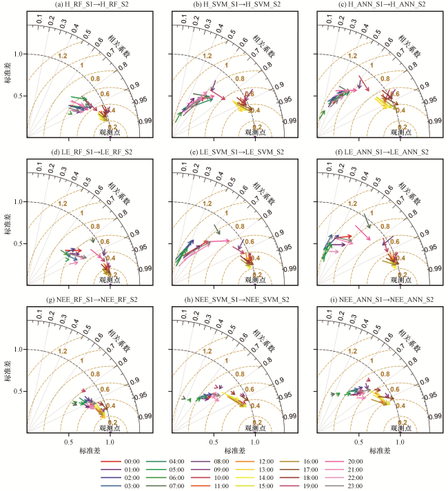
图3 两种方案下机器学习算法对感热通量、 潜热通量和净生态系统交换量模拟的泰勒图橙色虚线为均方根误差; 黑色实线为相关系数; 黑色虚线为标准差; 箭头起点(终点)位置对应S1(S2)方案模拟得到的均方根误差、 相关系数和标准差, 箭头指向观测点, 表示模拟效果提高 Fig.3 Taylor diagram showing change in machine learning algorithm performances when changing input variables.The orange dashed line is the root mean square error; the black solid line is the correlation coefficient; the black dashed line is the standard deviation.The starting (end) points position of the arrows represent root mean square error, correlation, and standard deviation for S1 (S2).If an arrow points toward observed values, it means model performance was improved.The colored line indicates each hour |
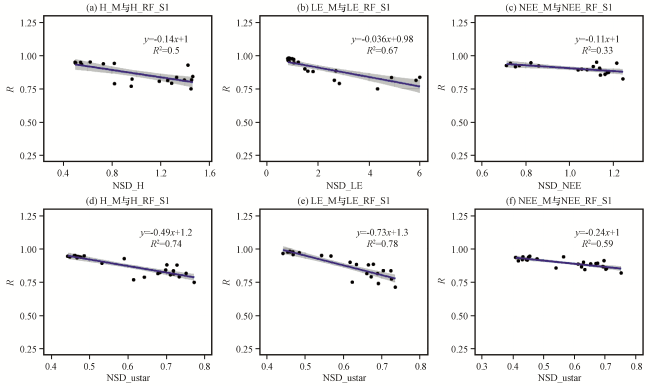
图4 小时尺度上机器学习算法模拟的感热通量、 潜热通量和净生态系统交换量与实测值的相关系数R随感热通量、 潜热通量、 净生态系统交换量(a~c)和摩擦速度(d~f)的归一化标准差的变化R代表相关系数; NSD代表归一化的标准差; ustar代表摩擦速度 Fig.4 Scatter plots of the correlation coefficient R between the sensible heat flux, latent heat flux and net ecosystem exchange volume simulated by the machine learning algorithm against the normalized sensible heat flux, latent heat flux, net ecosystem exchange volume (a~c) and the friction speed (d~f) on the hour scale. The R represents correlation coefficient. NSD represents normalized standard deviation; The ustar represent friction velocity |
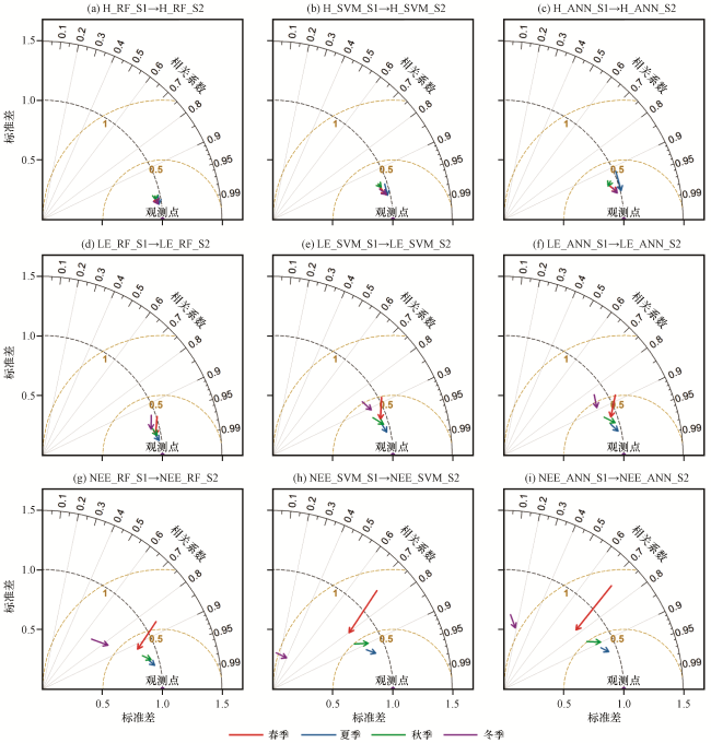
图5 两种方案下机器学习算法对感热通量、 潜热通量和净生态系统交换量模拟的泰勒图橙色虚线为均方根误差; 黑色实线为相关系数; 黑色虚线为标准差; 箭头起点(终点)位置对应S1(S2)方案模拟得到的均方根误差、 相关系数和标准差, 箭头指向观测点, 表示模拟效果提高 Fig.5 Taylor diagram showing change in machine learning algorithm performances when changing input variables.The orange dashed line is the root mean square error; the black solid line is the correlation coefficient; the black dashed line is the standard deviation.The starting (end) points position of the arrows represent root mean square error, correlation, and standard deviation for S1 (S2).If an arrow points toward observed values, it means model performance was improved.The colored line indicates each hour |
3.3 环境变量的依赖性和重要性
3.4 插补方法的选择对年累积量的影响
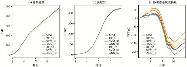


图8 2016年感热通量、 蒸散发、 和净生态系统交换累积量的变化Fig.8 Cumulative sensible heat flux, evapotranspiration and net ecosystem exchange over the course of 2016 |
表4 感热通量、 蒸散发和净生态系统交换插补后的累积量Table 4 The cumulative amount of sensible heat flux, evapotranspiration and net ecosystem exchange after interpolation |
| 项目 | 1月 | 2月 | 3月 | 4月 | 5月 | 6月 | 7月 | 8月 | 9月 | 10月 | 11月 | 12月 | 全年 |
|---|---|---|---|---|---|---|---|---|---|---|---|---|---|
| H_MDS/MJ | 63.9 | 95.8 | 114.2 | 121.7 | 96.0 | 66.2 | 56.9 | 84.0 | 56.6 | 65.5 | 67.7 | 64.2 | 952.6 |
| H_RF_S1/MJ | 64.0 | 96.2 | 114.6 | 121.1 | 99.0 | 66.2 | 57.3 | 84.5 | 56.9 | 65.7 | 68.2 | 64.0 | 957.9 |
| H_SVM_S1/MJ | 64.0 | 96.0 | 114.4 | 121.0 | 97.7 | 66.0 | 57.0 | 84.3 | 56.8 | 65.5 | 68.2 | 64.2 | 955.2 |
| H_ANN_S1/MJ | 63.9 | 95.8 | 114.3 | 121.2 | 99.4 | 66.9 | 57.4 | 84.6 | 57.4 | 65.9 | 67.9 | 64.2 | 958.9 |
| H_RF_S2/MJ | 64.5 | 96.3 | 115.2 | 121.8 | 96.3 | 66.6 | 57.4 | 84.7 | 57.2 | 66.2 | 68.7 | 65.0 | 959.9 |
| H_SVM_S2/MJ | 64.5 | 96.7 | 114.9 | 122.0 | 95.5 | 66.5 | 57.2 | 84.5 | 57.0 | 65.9 | 68.7 | 64.9 | 958.3 |
| H_ANN_S2/MJ | 64.3 | 97.7 | 114.5 | 121.7 | 96.9 | 67.1 | 56.6 | 84.4 | 57.8 | 66.4 | 68.9 | 64.9 | 961.2 |
| ET_MDS/mm | 5.9 | 7.1 | 14.5 | 28.5 | 53.2 | 74.2 | 84.8 | 76.4 | 46.3 | 34.7 | 13.0 | 7.5 | 446.1 |
| ET_RF_S1/mm | 5.9 | 7.5 | 14.4 | 28.0 | 52.2 | 73.8 | 84.2 | 76.6 | 45.5 | 33.8 | 13.0 | 7.5 | 442.4 |
| ET_SVM_S1/mm | 5.8 | 7.5 | 14.6 | 28.2 | 51.6 | 73.4 | 83.8 | 76.4 | 45.0 | 33.8 | 13.1 | 7.6 | 441.0 |
| ET_ANN_S1/mm | 6.1 | 7.2 | 14.6 | 28.3 | 51.9 | 73.6 | 84.2 | 76.8 | 45.4 | 34.0 | 12.9 | 7.4 | 442.5 |
| ET_RF_S2/mm | 5.9 | 7.1 | 14.2 | 28.1 | 53.7 | 74.1 | 85.1 | 76.6 | 46.4 | 34.3 | 12.9 | 7.5 | 445.9 |
| ET_SVM_S2/mm | 5.8 | 7.3 | 14.1 | 28.2 | 53.5 | 74.3 | 84.7 | 76.5 | 46.1 | 34.1 | 12.9 | 7.5 | 445.0 |
| ET_ANN_S2/mm | 5.9 | 7.2 | 14.2 | 28.5 | 53.8 | 74.5 | 84.9 | 76.3 | 46.2 | 34.5 | 12.8 | 7.3 | 446.1 |
| NEE_MDS/(gC·m-2) | 13.8 | 11.7 | 16.5 | 4.0 | -16.1 | -52.3 | -90.9 | -31.9 | -25.8 | 4.2 | 21.6 | 21.2 | -124.2 |
| NEE_RF_S1/(gC·m-2) | 13.4 | 5.9 | 1.7 | 1.8 | -9.9 | -50.3 | -92.2 | -33.4 | -24.1 | 6.2 | 19.5 | 15.5 | -146.2 |
| NEE_SVM_S1/(gC·m-2) | 11.9 | 3.9 | 3.4 | 0.4 | -14.3 | -53.9 | -95.7 | -36.8 | -30.9 | 2.5 | 18.8 | 14.5 | -176.4 |
| NEE_ANN_S1/(gC·m-2) | 9.3 | 7.6 | 8.1 | 2.2 | -11.6 | -51.3 | -91.7 | -32.6 | -26.8 | 4.4 | 20.0 | 15.8 | -146.6 |
| NEE_RF_S2/(gC·m-2) | 15.7 | 13.7 | 20.8 | 8.1 | -7.9 | -50.9 | -86.8 | -30.5 | -20.0 | 7.0 | 23.0 | 26.8 | -81.2 |
| NEE_SVM_S2/(gC·m-2) | 16.5 | 14.5 | 17.6 | 5.3 | -13.4 | -54.7 | -91.7 | -35.3 | -27.9 | 2.0 | 21.3 | 26.1 | -120.0 |
| NEE_ANN_S2/(gC·m-2) | 2.4 | 3.5 | 13.9 | 7.5 | -10.2 | -54.4 | -89.7 | -30.5 | -26.5 | 3.9 | 20.5 | 10.1 | -149.7 |